Volume Calculation

10 Steps to Calculate a Volume in Agisoft Metashape with GCPs | Aerial Surveying

IMPORTANCE OF GROUND CONTROL POINTS:

Using Drone Photogrammetry Software Agisoft Metashape. The above Video, Outlines the 10 Easy Steps to Generate an Accurate Volume of a Stockpile, using Imported Ground Control Points.

In any Aerial Survey it is Imperative for the Surveyor to know the Exact Coordinates of Ground Control Points.

However, depending on what type of UAV you are using for the Survey; much Existing Data can be found to show that, when using an RTK Drone, the Accuracy does not always increase if GCP’s are Utilised.

TIP: ‘Main Reason why Mining Companies are Using Drones for Volume Calculations’

It is however, important to understand that without GCP’s an Aerial Survey could be missing out on other Vital Information, such as correct Scale and Orientation.

 In Agisoft Metashape the Process to work out the Volume Accurately includes the Creation of the following 4 Models:

• 1: Alignment of Photos
• 2: Creation of a Dense Cloud
• 3: Digital Elevation Model
• 4: Orthomosaic.

 ALIGN PHOTOS:

The Process of Photo Alignment in Agisoft can also be referred to as Splicing the Individual Photos together to create a Sparse Cloud of Common Points called Tie-In Points.

The Software Achieves this by first finding KEY POINTS; which is the number of Points Metashape will Extract from each photograph.

Prior to Photo Alignment, Photos must first be added, by Selecting: Workflow >> Add Photos

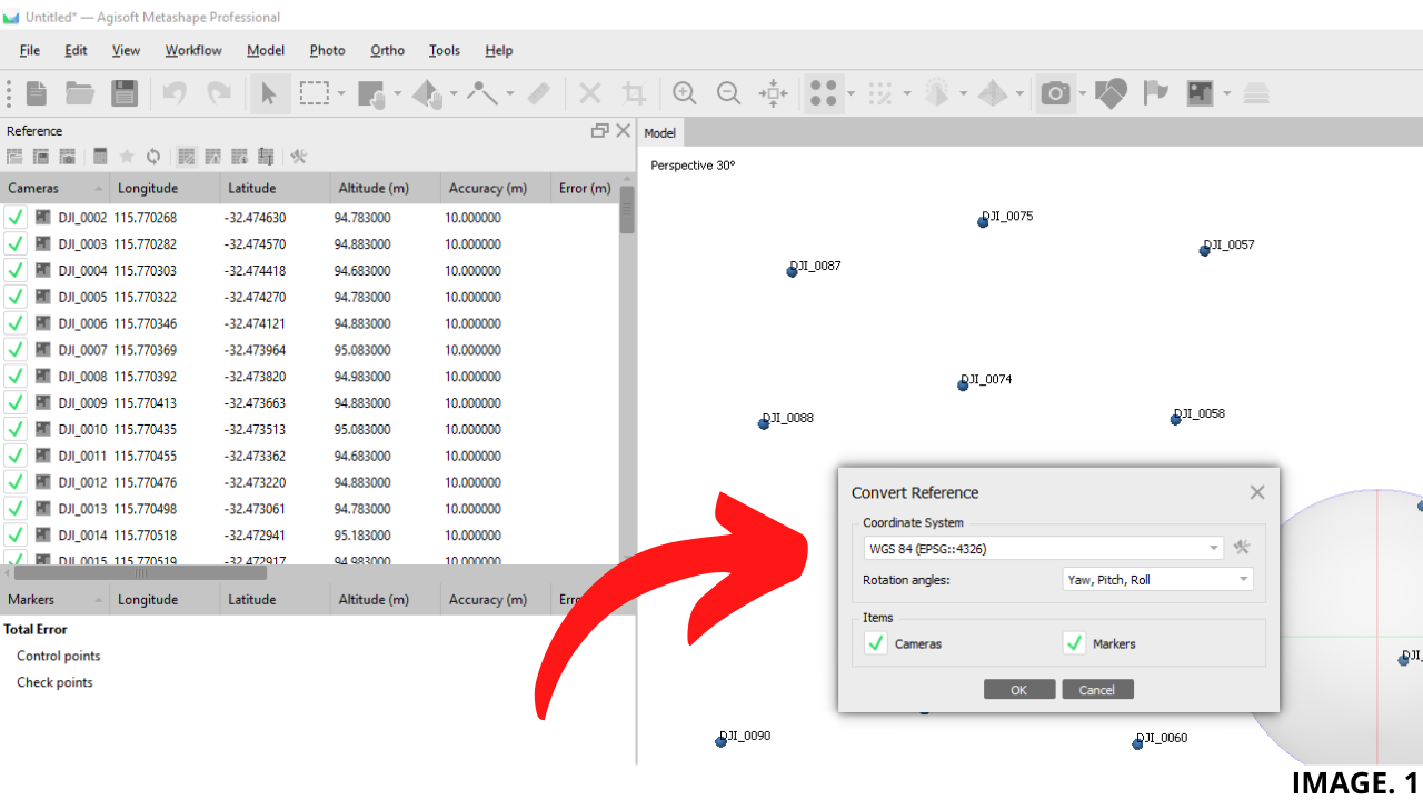
Then, it is an Important Step to Convert your captured photo Coordinates to the correct Local System. This would usually be from the WGS GPS Default Coordinates into your GCP Coordinate System.

Image. 1 shows this Option:

KEY & TIE POINT ALIGNMENT

The next part of the Photo Splicing is carried out by the TIE POINT ALIGNMENT; this is the amount of Matching Points that the Software Identifies in each Photograph.

The User can select the Amount of Points Metashape will search for in each step. By Default the Software Recommends:

Key Point Limit: 40,000

Tie Point Limit: 1,000

This means that Metashape will Extract 40,000 Points from each Photo and keep the Best Matching 1,000.

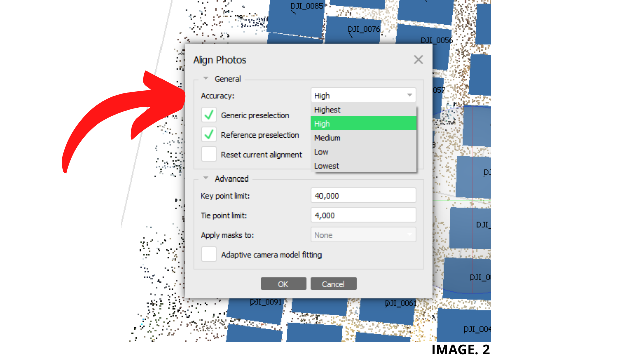
Accuracy can also be selected when Aligning Photos from:

• Highest (x4)
• High (Default)
• Medium (- x4)
• Low (- x16)
• Lowest (- x64)

As a Default, Agisoft uses HIGH Accuracy as the same Photo Resolution as the Photos collected in the Field. Where, HIGHEST Accuracy will upscale the Images by a Factor of 4. Heading Downscale from Highest each subsequent Option is then Reduced by a Factor of 4.

Image.2 shows Options for Photo Alignment:

GROUND CONTROL POINTS:

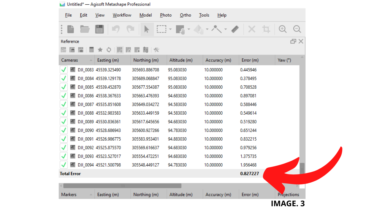
After Alignment is complete, you can check in the Top Left window, the current existing ‘Error Without Ground Control Points’. Image. 3 shows this:

The Next Step is to Import your Ground Control Points, this has to be a .CSV File. You must Check that your Ground Control Points are in the Correct Format, Press OK, then select, YES to ALL.

Now we can see the markers have appeared in the Model. We also notice that a lot of Error is still present; Therefore, the next Step is to Manually Align the Markers to our Ground Control Points.

TIP: ‘What is the Optimal Amount of Ground Control Points for an Accurate Survey ?’

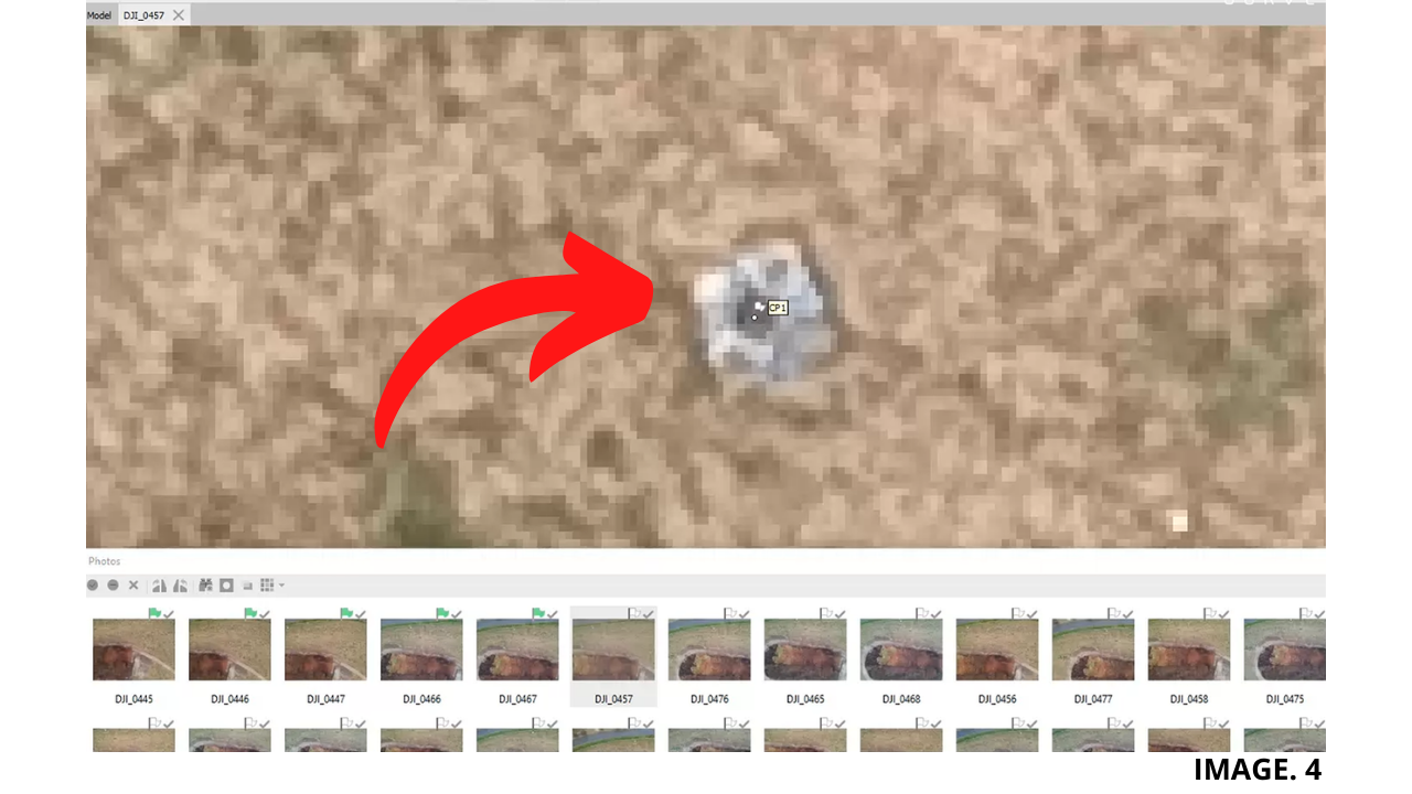
Any Photo that now shows a White Flag, actually contains a Marker that needs to be Aligned Manually to a Ground Control Point. After you Manually Align Two Markers, you will notice that the rest of the Photos Automatically Align their Markers very close to the Ground Control Points.

When you Right Click on a Ground Control Point in the Left Hand Table, and Select: ‘Filter Photos by Markers’; You can now see, each Photograph has Aligned itself around the Marker.

This Obviously makes it easier to click through each Photograph and Align them Quicker. The Next Step is to go through and Check EACH Photograph. You must also remember to repeat this process for EVERY Ground Control Point that you have.

Image. 4 Shows the Manual Alignment of Markers to Control Points:

REDUCED ERROR AND OPTIMISE CAMERAS:

The Video Example, uses only TWO Ground Control Points, which is of course not Optimal, and so to get better Accuracies you will want to use at least TEN Ground Control Points. Now that everything has been Aligned, we can now select the ‘Update’ button.

Once Updated, we can now see that the Error has been transferred from the Ground Control Point Window to the Original Photograph Window.

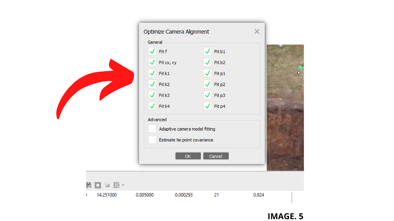
The remaining Error is also a ‘Residual’ Error, and we will further reduce it by Optimising our Camera Alignment. We will now select the ‘Optimise Camera Button’, select ALL Cameras, then OK.

Then, once the Software has finished Optimising, you will see a TOTAL Residual ‘Error’, in our Ground Control Point Window.

Image. 5 Shows the Table for Optimising Cameras:

DENSE CLOUD:

Now that we have Reduced the Error, we can continue with the Workflow Process. We must now create the Dense Cloud Model.

TIP: ‘Check the Difference between Drone Data, Point Clouds & Accurate Georeferenced 3D Models’

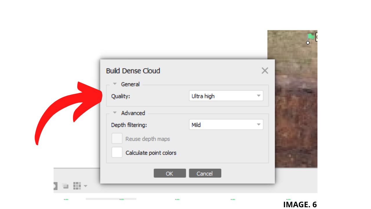
The Dense Cloud first gives you the Option to Choose a Quality Setting. As a Default, we will use Metashape on Ultra High, for a Ratio of 1:1 Processing. We can then Futher Reduce the Quality by a Factor of 2 for every other Setting.

As an Example of the Dense Cloud Quality Settings; if we select Ultra High, we produce 1 Million Points, then High Will Produce 500,000 Points.

We see the other Ratios are given as:

Ultra High: 1:1

High: 1:2

Medium: 1:4

Low: 1:8

Lowest: 1:16

The Next Option that we will Select in the Dense Cloud Tab, is the Depth Filtering Option. If we set this Option to AGGRESIVE (Highest), we will Filter or Remove most of the Points which do not appear to be connected to a Main Surface.

TIP: ‘Check how to Process Millions of Points from Agisoft to Surpac, in a .asc Point Cloud’

We will generally set this to the Lowest Setting of MILD, unless we want to Filter away things like Leaves/Plants etc.

Image. 6 Shows the Options used for a Dense Cloud:

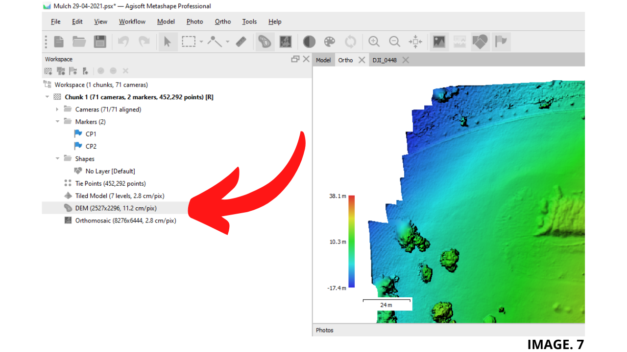
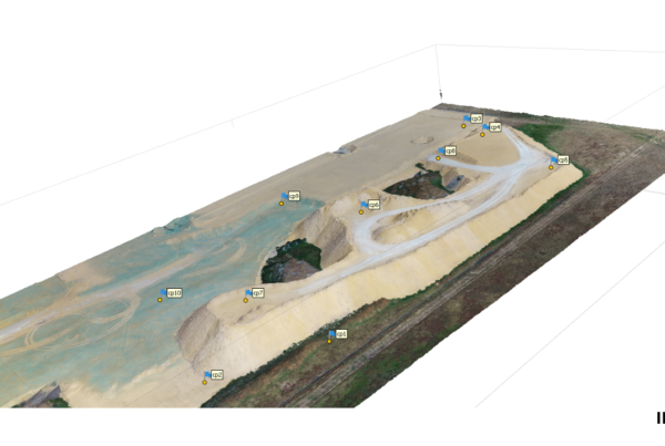
DIGITAL ELEVATION MODEL (DEM):

In order to Calculate the Volume of the Stockpile, it is now Necessary to Create a DEM or Digital Elevation Model. For more accurate results; we will Source the Data from the Dense Cloud. We willalso Select the correct Coordinate System.

TIP: ‘Look into some more Detail about DEM Volume Calculation’

The DEM in Metashape Graphically represents the Surveyed Terrain. The smaller the Raster Pixels, then the more Detailed the Model will be.

Image. 7 shows the location of the Size of the DEM Pixels:

ORTHOMOSAIC:

In Metashape, the Orthomosaic is not Necessary to Calculate the Volume, but can be very useful in Identifying certain Features in order to Correctly Map Out the Volume Base.

TIP: ‘Why Are Orthomosaics Important in Aerial Surveying?’

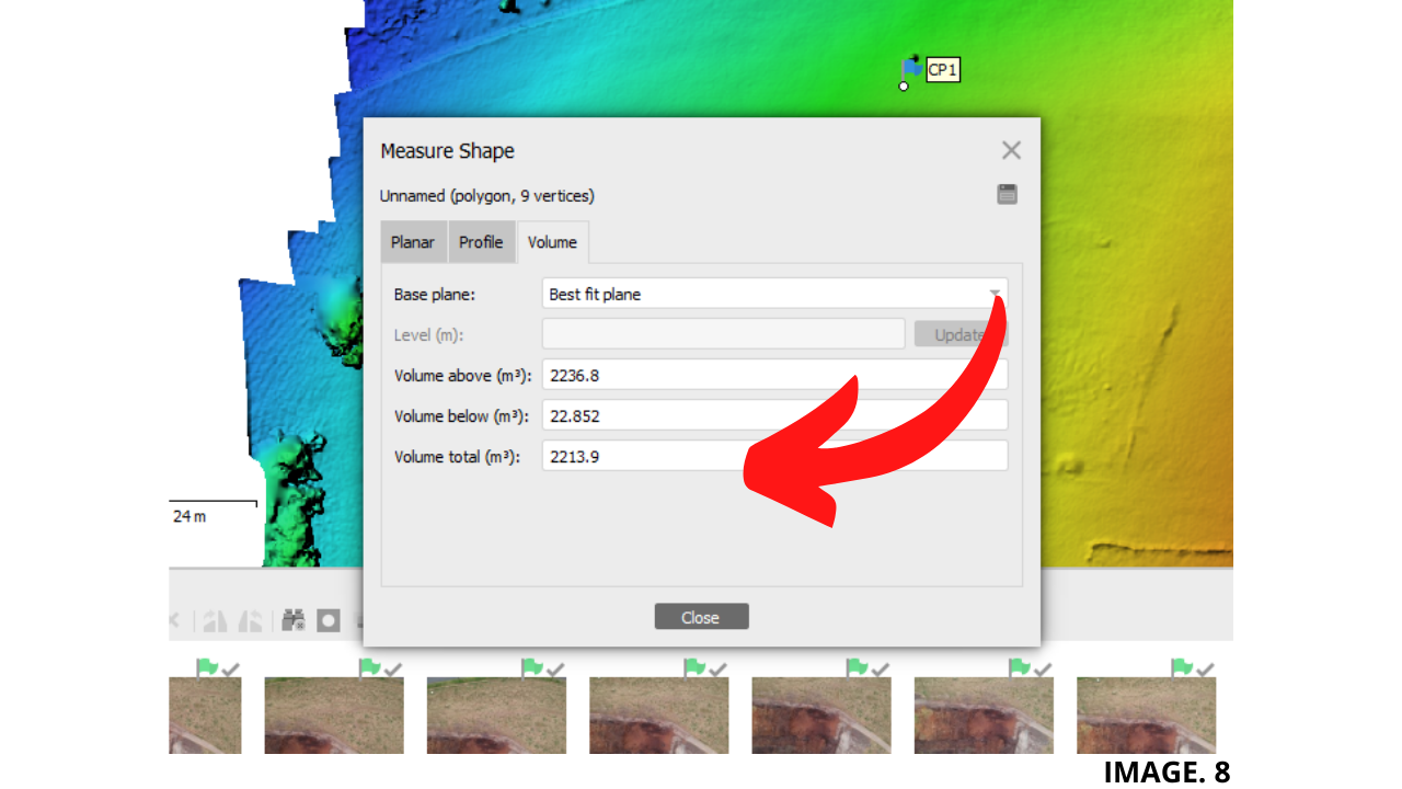
To Correctly find the Volume; select the Polygon Tool, and Draw a Polygon around the Stockpile Area that you want to measure. You can then select the, Orthomosaic to check if drawing your polygon in the correct Area.

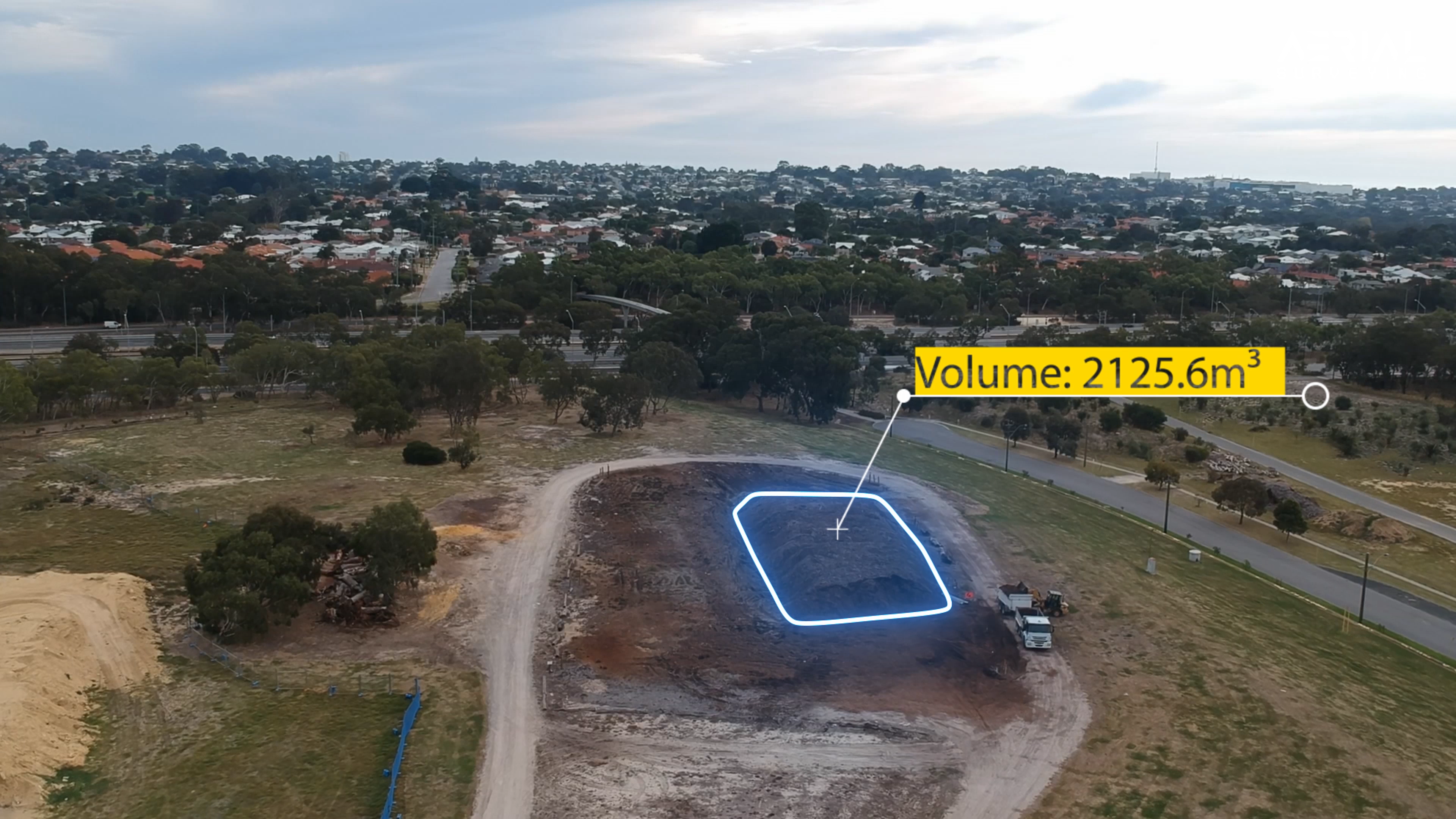
We find the VOLUME, by going back to the DEM Window, Right Clicking inside our Shape, Selecting Measure, Clicking on the Volume Tab; We can now see the Volume shown as a Total m³.

Image. 8 Shows the Total Volume in the Tab:

IN CONCLUSION:

Most Mining Companies today are still using the Above Method and Software to Calculate their Volume Control. It is therefore helpful for Educational purposes, Software such as Agisoft Metashape is essential Skill to learn in Aerial Surveying.

We Aim to bring more of this type of Content in the Future.